Modelling an inverted pendulum – deriving a mathematical model

This is part of a series of posts covering the development of a self-balancing robot:

Aim

Accurately model an inverted pendulum to use for control algorithms development for physical implementation.

Personal goal: refresh basic understanding of modelling and control.

Newton’s law

The cornerstone for obtaining a mathematical model, or the equations of motion for any mechanical system is Newton’s law [1]

$F=ma$

F = the vector sum of all forces applied to each body in the system, newtons [N]
a = vector acceleration of each body with respect to an inertial reference frame, m/s²
m = mass of body, kg

The application of Newton’s law to one-dimensional rotational systems requires the equation to be modified to

$M = I\alpha$

M = the sum of all external moments about the centre of mass of a body, N.m
I = the body’s mass moment of inertia about it’s centre of mass, kg.m²
α = the angular acceleration of the body, rad/s²

Free body diagram

Inverted pendulums usual take one of three forms, either an inverted pendulum on a linear track, inverted pendulum on a cart or a self-balancing robot.

Equations of motion

With Newton’s law and the self-balancing robot’s free body diagram we can go ahead and write the equations of motion for the system. In this example, the equations of motion for the x and y directions will be derived using the free body diagram of a pendulum on a cart.

X-axis

Starting with the x-axis and $F=ma$ , we can consider the self-balancing robot consisting of a cart (the wheels and motors) with mass M and a pendulum (everything else free to rotate in respect to the wheel and motors) with mass m. The pendulum’s mass is located a distance $l$ from the pivot point. For the self-balancing robot the pivot point is the axle.

Summing the forces acting on the robot in the x-direction we have

$F=u-b\dot{x}$

u = the force provided by the motors and wheels to move the robot in the x-direction
b = friction constant
$\dot{x}$ = first derivative of the robot’s position, it’s velocity

Considering the cart part and the pendulum part we have
$M$ = cart’s mass
$x$ = cart’s position
$m$ = pendulum’s mass
$x_p = x+l\sin(\theta)$ = pendulum’s position

We see the pendulum’s position is dependent on the angle $\theta$ and the cart’s position. With all this information we can now complete the equations of motion in the x-direction for the robot. Starting with Newton’s equation

$F=ma$

$F$ we have determined consists of the force provided by the wheels/motors and the friction the wheels encounter with the surface

$F=ma$
$u-b\dot{x}=ma$

The mass and acceleration, $ma$ , is that of the combined cart and pendulum. This can be split into the cart’s mass and acceleration and the pendulum’s mass and acceleration resulting in

$u-b\dot{x}=ma$
$u-b\frac{dx}{dt}=M\frac{d^2 x}{dt^2} + m\frac{d^2 x_p}{dt^2}$

$\frac{d^2 x_c}{dt^2}$ = cart’s acceleration
$x$ = cart’s position
$\frac{d^2 x_p}{dt^2}$ = pendulum’s acceleration
$x_p$ = pendulum’s position

We have already determined the pendulum’s position, $x_p$ , relative to $x$ above. This can now be added to the equation to complete the equation of motion.

$u-b\frac{dx}{dt}=M\frac{d^2 x}{dt^2} + m\frac{d^2}{dt^2}(x+l\sin(\theta))$

With the differentiation sum rule this is split into
$u-b\frac{dx}{dt}=M\frac{d^2 x}{dt^2} + m\frac{d^2x}{dt^2}+ m\frac{d^2}{dt^2}(l\sin(\theta))$

which can then be rewritten as

$u-b\frac{dx}{dt}=(M+m)\frac{d^2 x}{dt^2}+ m\frac{d^2}{dt^2}(l\sin(\theta))$

As $l$ is a constant it can be moved from within the differentiation to join $m$ . For easier referencing later, let’s call this equation 1.

$u-b\frac{dx}{dt}=(M+m)\frac{d^2 x}{dt^2}+ ml\frac{d^2}{dt^2}(\sin(\theta))$ [1]

Almost there, only the second derivative of $sin(\theta)$ left to calculated using the chain rule. The first derivative is calculated as

$\frac{d}{dt}\sin(\theta)=\cos(\theta).\dot{\theta}$

This is differentiated once again using the differentiation product and chain rules

$\frac{d^2}{dt^2}\sin(\theta)=\frac{d}{dt}(\cos(\theta)).\dot{\theta})$

$\frac{d^2}{dt^2}\sin(\theta)=\dot{\theta}.\frac{d}{dt}(\cos(\theta))+\cos(\theta)\frac{d}{dt}\dot{\theta}$

$\frac{d^2}{dt^2}\sin(\theta)=-\dot{\theta}\sin(\theta)\dot{\theta}+\cos(\theta).\ddot{\theta}$

$\frac{d^2}{dt^2}\sin(\theta)=-\dot{\theta}^2.\sin(\theta)+\cos(\theta).\ddot{\theta}$

All of this can now be plugged back into equation 1 to finish the equation of motion in the x-direction.

$u-b\frac{dx}{dt}=(M+m)\frac{d^2 x}{dt^2}+ ml(-\dot{\theta}^2.\sin(\theta)+\cos(\theta).\ddot{\theta})$

$u-b\dot{x}=(M+m)\ddot{x}- ml.\sin(\theta).\dot{\theta}^2+ml.\cos(\theta).\ddot{\theta}$ [2]

Y-axis

The equation for motion in the y-direction is a bit easier. The free body diagram we are working with is all the way back at the top of the post. Let’s show it again and consider it for the y-direction.

Free body diagram of cart and inverted pendulum

There is a single force acting in the y-direction, the pendulum’s weight. Knowing this suggests that the equation of motion in this direction will be very easy, but this is not to be the case. Although the force is in one direction the resulting movement will be in both the x and y-directions as the pendulum rotates about the pivot point. To make life a bit easier for ourselves it is easier to write the equation of motion in the direction of travel of the pendulum indicated by the red vector in the figure below.

Calculating moment about pendulum’s centre of mass

We start again with Newton’s second law. The force F along the red vector is

$F=mg\sin\theta$

As we have written the force along red vector, we need to do the same with the the acceleration vector $a$ . Previously we have already determined the pendulum’s x-position $x_p$ . We now do the same for its y-position $y_p$ .

$x_p = x+l\sin(\theta)$ = pendulum’s x-position

$y_p = l\cos(\theta)$ = pendulum’s y-position

The x and y-positions are then written as their components along the red vector.

$F = ma$

$mg\sin\theta = m\cos(\theta)\frac{d^2}{dt^2}x_p-m\sin(\theta)\frac{d^2}{dt^2}y_p$

Replacing $x_p$ and $y_p$ with their definition we get

$mg\sin\theta = m\cos(\theta)\frac{d^2}{dt^2}(x+l\sin(\theta))-m\sin(\theta)\frac{d^2}{dt^2}(l\cos(\theta))$

Luckily we have already calculated the second order derivative of $x_p$ and can reuse it here. Along with calculating the second order derivative of $y_p$ we get

$mg\sin(\theta) = m\cos(\theta)\frac{d^2}{dt^2}(x+l\sin(\theta)) - m\sin(\theta)\frac{d^2}{dt^2}(l\cos(\theta))$

$mg\sin(\theta) = m\cos(\theta) . (\ddot{x}+l.\cos(\theta).\ddot\theta-l\sin(\theta).\dot\theta^2) - ml\sin(\theta).(-\sin(\theta).\ddot{\theta}-\cos(\theta).\dot{\theta}^2)$

$mg\sin(\theta) = m\ddot{x}\cos(\theta) + ml\cos^2(\theta).\ddot{\theta} - ml\sin(\theta)\cos(\theta).\dot{\theta}^2 + ml\sin^2(\theta).\ddot{\theta} + ml\sin(\theta)\cos(\theta).(\dot\theta)^2$

This can be simplified to equation 3, the equation of motion in the y-direction. The simplification is achieved by two of the terms in the equation above adding to 0 and using the identity below

$1 = \cos^2(\theta) + \sin^2(\theta)$

$g\sin(\theta) = \ddot{x}\cos(\theta) + l\ddot{\theta}$ [3]

Linearisation

Both equations [2] and [3] are clearly non-linear. While we can attempt to do some non-linear control, for now it is best to keep things simple. As we want to balance the robot, we wish for the value of $\theta$ to be around zero. We will linearise the equations around this point. Later on when we feel brave we can linearise at some other points as well and maybe use gain scheduling for control over a wider angle range, but later.

Linearising around $\theta$ close to zero degrees we can do the following approximations

$\sin(\theta) \approx \theta$

$\cos(\theta) \approx 1$

X-axis

Starting with the equation of motion in the x-direction, using these approximations we can take equation 2

$u-b\dot{x}=(M+m)\ddot{x}- ml.\sin(\theta).\dot{\theta}^2+ml.\cos(\theta).\ddot{\theta}$ [2]

and simplify it to

$u-b\dot{x}=(M+m)\ddot{x}- ml\theta.\dot{\theta}^2+ml.\ddot{\theta}$ [4]

We are still left with $\dot{\theta}^2$ in the equation that can make life difficult. As we have already said the angle should remain 0, we can also assume that the angular speed will be close to 0, i.e. before we have significant angular speed, we aim to control the angle and bring it back to zero. Thus, if we take $\dot{\theta}^2 = 0$ we can further simplify the equation to

$u-b\dot{x}=(M+m)\ddot{x}+ml.\ddot{\theta}$ [5]

Y-axis

Moving to the equation of motion in the y-direction, doing the same with equation 3

$g\sin(\theta) = \ddot{x}\cos(\theta) + l\ddot{\theta}$ [3]

we get

$g\theta = \ddot{x} + l\ddot{\theta}$ [6]

State space representation

To complete the modelling of the self-balancing robot I will simulate its behaviour, probably using MATLAB Simulink. It can also be done in Python, C, or really anything else, including Excel. The non-linear equations of motion we have derived above is also already sufficient for that purpose, but ultimately the goal is to develop a control strategy. To assist it makes sense to represent the linearised equation of motion in state-space as well as a transfer function. Having both state-space and transfer function representations will allow us to later explore different methods of controlling the robot.

So, what is the state-space representation? Wikipedia or any textbook does a much better job at explaining this than I ever will, but in short, from Wikipedia, it is a mathematical model of a physical system as a set of input, output and state variables related by first order differential equations. The block diagram illustrates this statement.

The output, $y$ , can be written as the sum of the product of the input, $u$ , and the vector $D$ and the product of state, $x$ and vector $D$ . The state $\dot{x}$ in turn is writen as the sum of product of the input, $u$ , and the vector $B$ and the product of state $x$ and vector $A$ . This is written as

$\begin{bmatrix} \dot{x} \end{bmatrix} = \begin{bmatrix} A \end{bmatrix}\begin{bmatrix} x \end{bmatrix} + \begin{bmatrix} B \end{bmatrix}\begin{bmatrix} u \end{bmatrix}$

$\begin{bmatrix} y \end{bmatrix} = \begin{bmatrix} C \end{bmatrix}\begin{bmatrix} x \end{bmatrix} + \begin{bmatrix} D \end{bmatrix}\begin{bmatrix} u \end{bmatrix}$

With this limited background on the state space representation we proceed to writing the state space representation of our linearised equations of motion.

First we define our state variables

$x_1 = \theta$

$x_2 = \dot{\theta}$

$x_3 = x$

$x_4 = \dot{x}$

With the state space representation, we will write our equation of motion in the following form leaving us to calculate the values of the matrices A, B, C and D.

$\begin{bmatrix} \dot{x_1} \\ \dot{x_2} \\ \dot{x_3} \\ \dot{x_4}\end{bmatrix} = \begin{bmatrix} A \end{bmatrix}\begin{bmatrix} x_1 \\ x_2 \\ x_3 \\ x_4 \end{bmatrix} + \begin{bmatrix} B \end{bmatrix}\begin{bmatrix} u \end{bmatrix}$

The outputs of the system we are interested in are position $x$ and angle $\theta$ . We have already defined these as 2 of our state variables therefor we already have the matrices C and D defined:

$\begin{bmatrix} y_1 \\ y_2 \end{bmatrix} = \begin{bmatrix} \theta \\ x \end{bmatrix} = \begin{bmatrix} x_1 \\ x_3 \end{bmatrix}$

$\begin{bmatrix} y_1 \\ y_2 \end{bmatrix} = \begin{bmatrix} C \end{bmatrix}\begin{bmatrix} x \end{bmatrix} + \begin{bmatrix} D \end{bmatrix}\begin{bmatrix} u \end{bmatrix}$

$\begin{bmatrix} y_1 \\ y_2 \end{bmatrix} = \begin{bmatrix} 1 & 0 & 0 & 0 \\ 0 & 0 & 1 & 0 \end{bmatrix}\begin{bmatrix} x_1 \\ x_2 \\ x_3 \\ x_4 \end{bmatrix} + \begin{bmatrix} 0 \end{bmatrix}\begin{bmatrix} u \end{bmatrix}$

Next, we need to determine the values of the A and B matrices. This can be done by solved using the linearised equations 5 and 6 describing the motion in both the x and y-direction.

$u-b\dot{x}=(M+m)\ddot{x}+ml.\ddot{\theta}$ [5]

$g\theta = \ddot{x} + l\ddot{\theta}$ [6]

Some mathenatical manipulation is required. Taking equation 5 we can rewrite this to

$u-b\dot{x}=M\ddot{x}+m\ddot{x}+ml.\ddot{\theta}$

$u-b\dot{x}=M\ddot{x}+m(\ddot{x}+l\ddot{\theta})$

We notice $\ddot{x}+l\ddot{\theta}$ is already defined in equation 6 to be equal to $g\theta$ . Replacing $\ddot{x}+l\ddot{\theta}$ with $g\theta$ we get

$u-b\dot{x}=M\ddot{x}+mg\theta$

With this we determine $\ddot{x}$

$M\ddot{x} = u-b\dot{x} - mg\theta$

$\ddot{x} = \frac{1}{M}u - \frac{b}{M}\dot{x} - \frac{mg}{M}\theta$ [7]

This we can write in terms of our state variables

$\dot{x_4} = \frac{1}{M}u - \frac{b}{M}x_4 - \frac{mg}{M}x_1$ [8]

The only unknown to complete our state space representation now is $\dot{x_2}$ better known as $\ddot{\theta}$ . As we now know what $\\ddot{x}$ is, see equation 7 above, we can just pop that back into equation 6 to determine $\ddot{x}$

$g\theta = \ddot{x} + l\ddot{\theta}$ [6]

$g\theta = \frac{1}{M}u - \frac{b}{M}\dot{x} - \frac{mg}{M}\theta + l\ddot{\theta}$

$l\ddot{\theta} = g\theta - \frac{1}{M}u + \frac{b}{M}\dot{x} + \frac{mg}{M}\theta$

$\ddot{\theta} = \frac{g}{l}(1 + \frac{m}{M})\theta - \frac{1}{Ml}u + \frac{b}{Ml}\dot{x}$

$\ddot{\theta} = g\frac{M+m}{Ml}\theta - \frac{1}{Ml}u + \frac{b}{Ml}\dot{x}$

This we can write in terms of our state variables

$\dot{x_2} = g\frac{M+m}{Ml}x_1 - \frac{1}{Ml}u + \frac{b}{Ml}x_4$ [9]

With that we have all the information we need about our state variables

$\dot{x_1} = x_2$

$\dot{x_2} = g\frac{M+m}{Ml}x_1 + \frac{b}{Ml}x_4 - \frac{1}{Ml}u$

$\dot{x_3} = x_4$

$\dot{x_4} = - \frac{mg}{M}x_1 - \frac{b}{M}x_4+ \frac{1}{M}u$

Writing this in matrix form, along with the output in matrix form we already done before, we complete the state space representation.

$\begin{bmatrix} \dot{x_1} \\ \dot{x_2} \\ \dot{x_3} \\ \dot{x_4}\end{bmatrix} = \begin{bmatrix} 0 & 1 & 0 & 0 \\ g\frac{M+m}{Ml} & 0 & 0 & \frac{b}{Ml} \\ 0 & 0 & 0 & 1 \\ - \frac{mg}{M} & 0 & 0 & - \frac{b}{M} \end{bmatrix}\begin{bmatrix} x_1 \\ x_2 \\ x_3 \\ x_4 \end{bmatrix} + \begin{bmatrix} 0 \\ - \frac{1}{Ml} \\ 0 \\ \frac{1}{M} \end{bmatrix}\begin{bmatrix} u \end{bmatrix}$ [10]

Transfer functions

Writing the transfer function should be a little bit easier, most of what we need we have already calculated. The transfer function takes the equations of motion and write them as a function of the output to the input, that is $\frac{Y(s)}{U(s)}$ with $Y(s)$ the output and $U(s)$ the input. For the self-balancing robot, we will have two transfer functions, one translating the input $u$ to the angle output $\theta$ and another translating input $u$ to the position output $x$ .

The Laplace transform is vital tool to solve differential equations and for us to write the transfer functions . We will not go into detail of the function but is recommended to read and understand its purpose.

It is worth noting that a transform exist to move between the state space representation and a transfer function.

Angle transfer function

To start we will determine the transfer function for the input $u$ to angle output $\theta$ . That is

$\frac{\theta(s)}{U(s)}$

To do this we take the Laplace transform of the equations of motion 5 and 6 calculated earlier and then solve them for $\theta$ . As a reminder our equations of motion are

$u-b\dot{x}=(M+m)\ddot{x}+ml.\ddot{\theta}$ [5]

$g\theta = \ddot{x} + l\ddot{\theta}$ [6]

Laplace transform

The Laplace transform of

$u-b\dot{x}=(M+m)\ddot{x}+ml\ddot{\theta}$ [5]

$U(s) - bX(s)s = (M+m)X(s)s^2 + ml\Theta(s)s^2$ [12]

Next we get the Laplace transform of

$g\theta = \ddot{x} + l\ddot{\theta}$ [6]

to be

$g\Theta(s) = X(s)s^2 + l\Theta(s)s^2$ [13]

We can rewrite equation 13 with $X(s)$ as the subject and to replace $X(s)$ in equation 12 to enable us to relate $\Theta(s)$ directly to $U(s)$ .

$g\Theta(s) = X(s)s^2 + l\Theta(s)s^2$ [13]

$X(s) = (\frac{g}{s^2} - l)\Theta(s)$ [14]

Let’s take equation 14 and replace $X(s)$ with this in equation 12

$U(s) - bX(s)s = (M+m)X(s)s^2 + ml\Theta(s)s^2$ [12]

$U(s) = (M+m)X(s)s^2 + bX(s)s + ml\Theta(s)s^2$

$U(s) = (M+m)(\frac{g}{s^2} - l)\Theta(s)s^2 + b(\frac{g}{s^2} - l)\Theta(s)s + ml\Theta(s)s^2$

This simplify to

$U(s) = \Theta(s)\frac{-lMs^3-bls^2+g(M+m)s+bg}{s}$

Which can now be written as our transfer function in equation 15

$\frac{\Theta(s)}{U(s)} = \frac{s}{-lMs^3-bls^2+g(M+m)s+bg}$

$\frac{\Theta(s)}{U(s)} = \frac{\frac{-1}{lM}s}{s^3+\frac{b}{M}s^2-\frac{g(M+m)}{lM}s-\frac{bg}{lM}}$ [15]

Position transfer function

The same steps as for the angle transfer function are followed to get the position transfer function. We already have the Laplace transforms and don’t need to do that again. Instead of rewriting equation 13 with $X(s)$ as the subject, rewrite it with $\Theta(s)$ as the subject.

$g\Theta(s) = X(s)s^2 + l\Theta(s)s^2$ [13]

$\Theta(s)(g-ls^2) = X(s)s^2$

$\Theta(s) = \frac{s^2}{g-ls^2}X(s)$ [16]

As before, we can now pop equation 16 back into equation 12 to replace $\Theta(s)}$

$U(s) - bX(s)s = (M+m)X(s)s^2 + ml\Theta(s)s^2$ [12]

$U(s) - bX(s)s = (M+m)X(s)s^2 + \frac{mls^2}{g-ls^2}X(s)s^2$

$U(s) = X(s)((M+m)s^2 + \frac{mls^4}{g-ls^2} + bs)$

This can be simplified to

$U(s) = X(s)(\frac{-lMs^4 - bls^3+g(M+m)s^2+bgs}{g-ls^2})$

And then rewritten as our transfer function in equation 17

$\frac{X(s)}{U(s)} = \frac{g-ls^2}{-lMs^4 - bls^3+g(M+m)s^2+bgs}$

$\frac{X(s)}{U(s)} = \frac{\frac{1}{M}s^2-\frac{g}{lM}}{s^4 + \frac{b}{M}s^3-\frac{g(M+m)}{lM}s^2-\frac{bg}{lM}s}$ [17]

Modelling

The last step in this post is to model our different interpretations of the equations of motion. Using tools such as MATLAB and MATLAB Simulink we can model the non-linear equations of motion (equations 2 and 3) with our linearised state-space and transfer function representation. Hopefully every line up and makes sense. If not, we will quickly see if we have made a mistake along the way.

Modelling non-linear equation of motion in Simulink

The non-linearised equations of motion, equations 2 and 3, are modelled in Simulink by rewriting the functions with $\ddot{x}$ and $\ddot{\theta}$ the subjects. We take our equations of motion

$u-b\dot{x}=(M+m)\ddot{x}- ml.\sin(\theta).\dot{\theta}^2+ml.\cos(\theta).\ddot{\theta}$ [2]

$g\sin(\theta) = \ddot{x}\cos(\theta) + l\ddot{\theta}$ [3]

and rearrange them to have

$\ddot{x} = \frac{u}{M+m} - \frac{b\dot{x}}{M+m} + \frac{ml\sin(\theta)\dot{\theta}^2}{M+m} - \frac{ml\cos(\theta)\ddot{\theta}}{M+m}$

$\ddot{\theta} = \frac{g\sin(\theta)}{l} - \frac{\cos(\theta)(u - b\dot{x} + ml\sin(\theta)\dot{\theta}^2 - ml\cos(\theta)\ddot{\theta})}{l(M+m)}$

Non-linear model of self-balancing robot

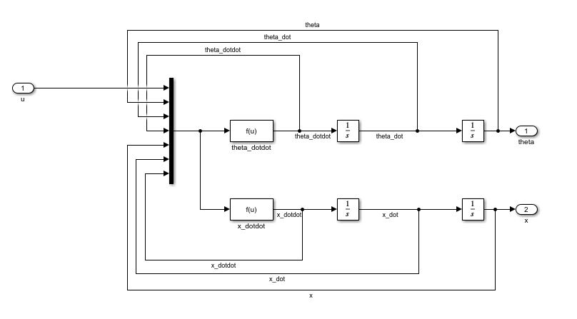
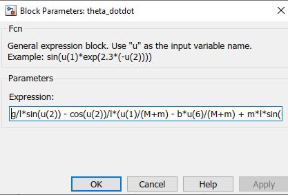
These equations are represented in the function Simulink block as below. We take the output of the $\ddot{\theta}$ and $\ddot{x}$ calculations and integrate them to get the first derivative and values of $\theta$ and $x$ . For simplicity the initial values of all integrals, the position and angle are set to zero.

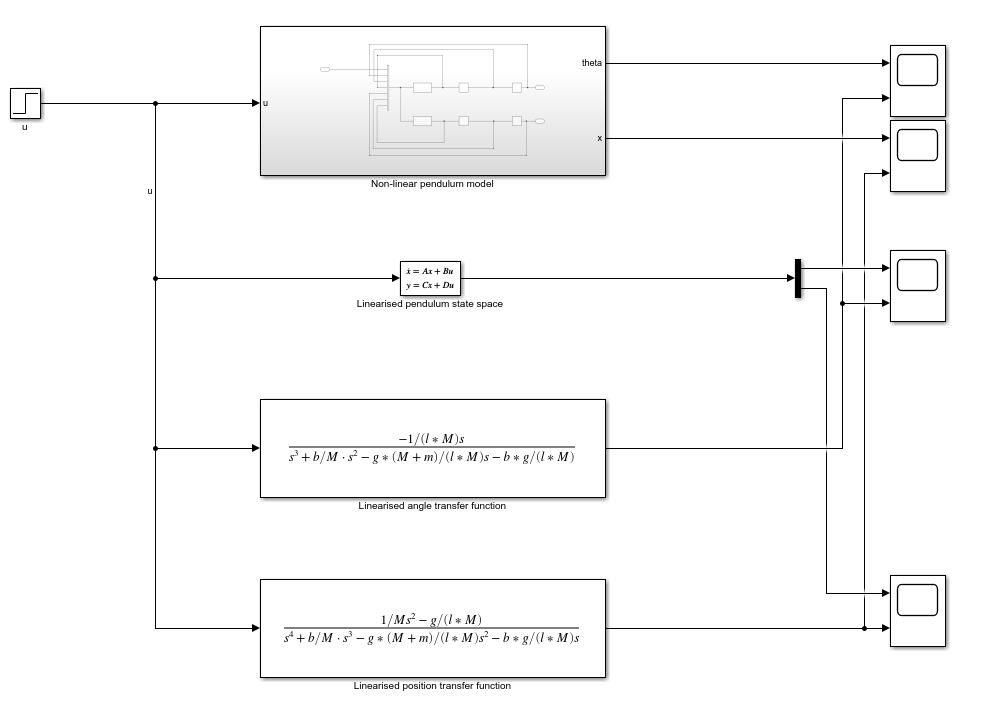
Entering non-linear calculation in function block

State space and transfer function representation in Simulink

The state space representation and transfer functions we have calculated are modelled in Simulink using the continuous State Space and transfer function blocks.

Simulink library blocks for transfer function and state space

Comparison

With all the different models and representations of our self-balancing robot we can compare the outputs.

As expected, the output of the two linearised representations, state space and transfer functions, match exactly. What is more interesting is to look at the difference between the non-linear and linear models

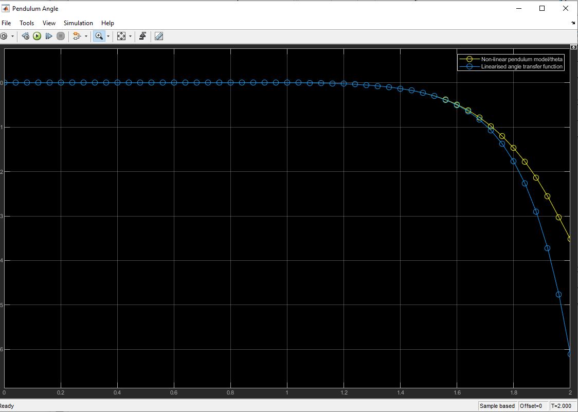
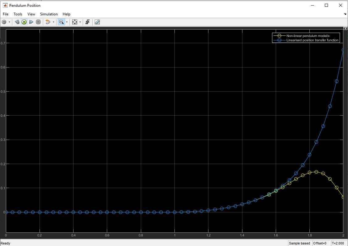
Pendulum angle output for a step input of U

Pendulum position output for a step input of U

The non-linear and linearised models compare very well for small values of $\theta$ validating the linearisation assumptions we have made. In the example we apply a 0.2 step at 1 s. The models compare well up until 1.6 s where they start to diverge. At this time the pendulum angle is -0.5 radians or -28 degrees.

Next steps

The next step is to use our linearised models to design a control system to control our self-balancing robot. Before this can be done the robot itself needs to be built to measure its properties to plug into the model.

The non-linear model will be used as the plant. It is worth noting that all the models we have made in this post make use of continuous time. Our control system will be running on discreet time. This is very important and will need to be taken into account during the design of our control strategy as well as modelling of the controller and plat later on.

Bibliography

Gene F Franklin, J David Powell and Abbas Emami-Naeni: Feedback control of dynamic systems. 4th Edition. Prentice Hall, 2002
P. Frankovský, L. Dominik, A. Gmiterko, I. Virgala: Modeling of two-wheeled self-balancing robot driven by DC gearmotors. Department of Mechatronics, Faculty of Mechanical Engineering, Technical University of Košice, 2017
Hanna Hellman, Henrik Sunnderman: Two-wheeled self-balancing robot. KTH Royal Institute of Technology, Stockholm, Sweden
State space representation, Wikipedia: https://en.wikipedia.org/wiki/State-space_representation

karooza.net

Covering electronics and coding for the hobbyist that wants to build everything

Modelling an inverted pendulum – deriving a mathematical model

Aim

Newton’s law

Free body diagram

Equations of motion

X-axis

Y-axis

Linearisation

X-axis

Y-axis

State space representation

Transfer functions

Angle transfer function

Laplace transform

Position transfer function

Modelling

Modelling non-linear equation of motion in Simulink

State space and transfer function representation in Simulink

Comparison

Next steps

Bibliography

Related

2 thoughts on “Modelling an inverted pendulum – deriving a mathematical model”

Leave a Reply Cancel reply