
In an upcoming project I want to experiment with image recognition and have a balance robot track and follow a colored ball. As a prelude to that project and to learn more about what is involved in terms of the image processing I came up with a smaller sub project. The idea is to just have a Raspberry Pi3 with a camera mounted on top of a small servo. The camera together with the Pi should then detect and track a yellow ball within the camera frame. Once the position of the ball is known, the Pi should also control the servo so that the camera keeps facing the ball.
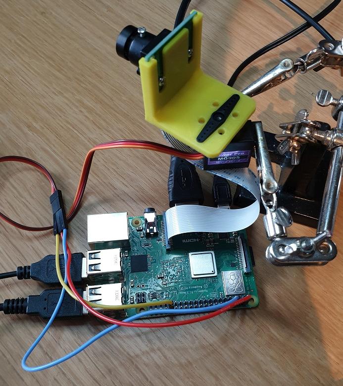
After doing a bit of research on how this can be achieved, I came up with a solution which I will share in this post. To keep it simple I used OpenCV and Python for programming the Pi. I have commented the code fairly well so will not describe each step, it is actually very self explanatory. The camera is a 5MP Raspberry Pi camera by WaveShare and the servo a MG90S by Tower Pro. Power for the servo is taken from the Pi’s 5V output and the servo signal line connected to GPIO12. The servo is held in place by some “soldering helping hands” and I printed a simple bracket to mount the camera to the servo.
Detecting the ball
So the approach I went with was to do blob detection on each frame that is read from the camera. If you haven’t heard of blob detection before, it basically does what it is called, it detects blobs or pixels which are grouped together. Once a blob (or multiple blobs) has been detected you can retrieve some additional information from it, like for example the size of the blob and where in the camera frame it is located.
OpenCV has a nice function that can do this for us, the only requirement is that it should be a black blob on a white background. So this means we should somehow isolate the ball (or rather the color of the ball) and then make it black and the background white. So in other words we will first create a black and white mask image from the frame we are processing and then perform blob detection on the mask.
HSV Color Space
Most likely you have heard or RGB (Red Green Blue) color model where each pixel is made up of a mixture of these three colors added together. The pixels we get from the camera are typically described in a RGB format which holds variables for the amount of red, green and blue for each pixel. Another way to represent the color of a pixel is by using the HSV color space.
When doing this we still have three components but they are now called Hue, Saturation and Value. Hue describes the primary color while Saturation the amount of gray making the color appear more or less faded.
The Value component describes the brightness or the color between completely black and the primary color. As you might have guessed, the reason why I am mentioning this is that we would need to transform from RGB to the HSV color space. The reason being that it’s easier to isolate colors when we work in the HSV color space.
Erode and Dilate
These two functions are morphology operators and very common in image processing. The erode function has the effect of eroding or removing parts of the image while the dilation function has the opposite effect of adding to parts of the image. These functions are more typically used on binary images, so images which are made up of only black and white pixels and will be used to clean up the image mask which we create.
Their function and behavior will become clearer later in the post.
Testing on still images
To get all the parameters tuned, it helps to first run the program on still images. I ran the program below which just provides a video stream from the camera. Then I aligned a couple of shots with my yellow ball in view and saved them as images.
import cv2

cap = cv2.VideoCapture(0)

while True:
    _, frame = cap.read()

    cv2.imshow("Video", frame)

    key = cv2.waitKey(1)
    if key == 27:
        break
Getting the HSV values
To make it easier to test different HSV values I created the following program:
import cv2
import numpy as np;

# Just dummy function for callbacks from trackbar
def nothing(x):
    pass

# Create a trackbar window to adjust the HSV values
# They are preconfigured for a yellow object
cv2.namedWindow("Tracking")
cv2.createTrackbar("LH", "Tracking", 20,255, nothing)
cv2.createTrackbar("LS", "Tracking", 120, 255, nothing)
cv2.createTrackbar("LV", "Tracking", 120, 255, nothing)
cv2.createTrackbar("UH", "Tracking", 49, 255, nothing)
cv2.createTrackbar("US", "Tracking", 255, 255, nothing)
cv2.createTrackbar("UV", "Tracking", 255, 255, nothing)

# Read test image
frame = cv2.imread("blob5.jpg")

while True:
    # Convert to HSV colour space
    hsv = cv2.cvtColor(frame, cv2.COLOR_BGR2HSV)

    # Read the trackbar values
    lh = cv2.getTrackbarPos("LH", "Tracking")
    ls = cv2.getTrackbarPos("LS", "Tracking")
    lv = cv2.getTrackbarPos("LV", "Tracking")
    uh = cv2.getTrackbarPos("UH", "Tracking")
    us = cv2.getTrackbarPos("US", "Tracking")
    uv = cv2.getTrackbarPos("UV", "Tracking")

    # Create arrays to hold the minimum and maximum HSV values
    hsvMin = np.array([lh, ls, lv])
    hsvMax = np.array([uh, us, uv])

    # Apply HSV thresholds
    mask = cv2.inRange(hsv, hsvMin, hsvMax)

    # Uncomment the lines below to see the effect of erode and dilate
    #mask = cv2.erode(mask, None, iterations=3)
    #mask = cv2.dilate(mask, None, iterations=3)

    # The output of the inRange() function is black and white
    # so we use it as a mask which we AND with the orignal image
    res = cv2.bitwise_and(frame, frame, mask=mask)

    # Show the result
    cv2.imshow("Result view", res)

    # Wait for the escape key to be pressed
    key = cv2.waitKey(1)
    if key == 27:
        break

cv2.destroyAllWindows()
When you run the program it reads and shows the image, trackbars are then provided to adjust minimum and maximum HSV values. I played with these values until I could more or less isolate the ball from the rest of the image and then wrote the HSV values down for later use.
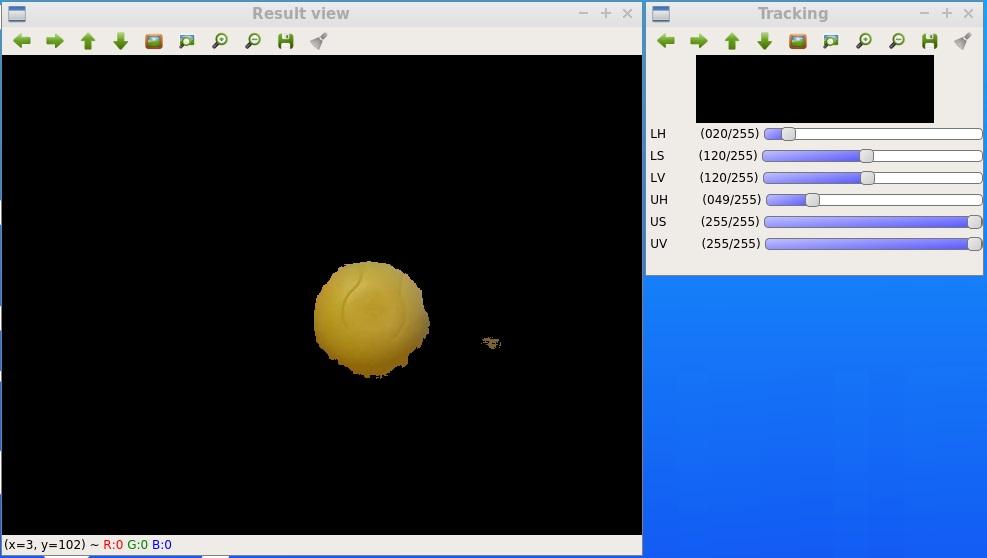
If you read through the program code you will see that I first create a mask which I then overlay (using AND logic) on top of the original image. The overlaid result allow you to easily see the effect of changing the HSV values but in the end it’s the mask that we are interested in and will use to do the blob detection.
Now is also a good time to better illustrate the effects of erode and dilate. To the right of the ball we can still see an unwanted part of the image showing through which we can remove with the erode function. In the program code I commented out the erode and dilute functions, if I now un-comment them and run it again you can see the effect:

We completely eroded the unwanted part away, but since the erode also shrinks our wanted part of the mask we dilate it afterwards to grow it out a bit again.
Detecting the blob
Now that we can create a mask which only allow our ball to be seen we are ready to perform the blob detection. As mentioned earlier, for the function to work we need a black blob on a white background and therefore first need to invert the mask.
Before we call the detector function we can also specify some parameters which it will consider while performing the detection. I added them in the program code so that you can see the options but I only enabled the size filter. After playing a bit with the size filter I picked some values that allowed the ball to be seen when it is close to the camera (and fairly large) as well as when it is further away (and a bit smaller). Normally the ball will be the main object in the frame and fairly large compared to other objects in the frame. By keeping the minimum size not to small I am trying to avoid other random objects which might pass through the mask from being detected.
When the blob detection is complete we receive a list of all the detected blobs and also their position on the image as well as size. Since I anticipate to only have one blob I only consider the first index in the list. Below is the program to detect the blob and give it’s position:
import cv2
import numpy as np;

# Font to write text overlay
font = cv2.FONT_HERSHEY_SIMPLEX

# Create lists that holds the thresholds
hsvMin = (20,120,120)
hsvMax = (49,255,255)

# Read test image
frame = cv2.imread("blob5.jpg")

# Convert to HSV
hsv = cv2.cvtColor(frame, cv2.COLOR_BGR2HSV)

# Apply HSV thresholds
mask = cv2.inRange(hsv, hsvMin, hsvMax)

# Erode and dilate
mask = cv2.erode(mask, None, iterations=3)
mask = cv2.dilate(mask, None, iterations=3)

# Adjust detection parameters
params = cv2.SimpleBlobDetector_Params()

# Change thresholds
params.minThreshold = 0;
params.maxThreshold = 100;

# Filter by Area.
params.filterByArea = True
params.minArea = 400
params.maxArea = 20000

# Filter by Circularity
params.filterByCircularity = False
params.minCircularity = 0.1

# Filter by Convexity
params.filterByConvexity = False
params.minConvexity = 0.5

# Filter by Inertia
params.filterByInertia = False
params.minInertiaRatio = 0.5

# Detect blobs
detector = cv2.SimpleBlobDetector_create(params)

# Invert the mask
reversemask = 255-mask

# Run blob detection
keypoints = detector.detect(reversemask)

# Get the number of blobs found
blobCount = len(keypoints)

# Write the number of blobs found
text = "Count=" + str(blobCount)
cv2.putText(frame, text, (5,25), font, 1, (0, 255, 0), 2)

if blobCount > 0:
    # Write X position of first blob
    blob_x = keypoints[0].pt[0]
    text2 = "X=" + "{:.2f}".format(blob_x )
    cv2.putText(frame, text2, (5,50), font, 1, (0, 255, 0), 2)

    # Write Y position of first blob
    blob_y = keypoints[0].pt[1]
    text3 = "Y=" + "{:.2f}".format(blob_y)
    cv2.putText(frame, text3, (5,75), font, 1, (0, 255, 0), 2)

    # Write Size of first blob
    blob_size = keypoints[0].size
    text4 = "S=" + "{:.2f}".format(blob_size)
    cv2.putText(frame, text4, (5,100), font, 1, (0, 255, 0), 2)

    # Draw circle to indicate the blob
    cv2.circle(frame, (int(blob_x),int(blob_y)), int(blob_size / 2), (0, 255, 0), 2)

# Show image
cv2.imshow("Blob detection", frame)
cv2.waitKey(0)
cv2.destroyAllWindows()
And the output when using it with one of the test images I took earlier:
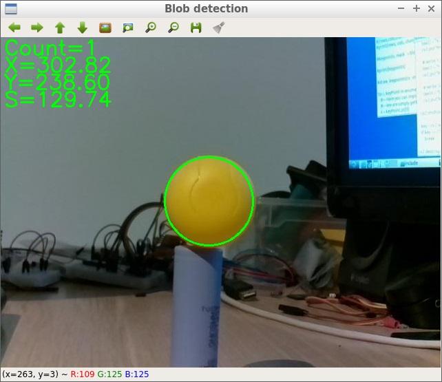
In the top left corner we have “Count” which is the number of blobs that has been detected as well as the X and Y pixel values of the center of the blob. The value of S is the diameter of the blob in pixels. Note that this is not the same as the area value we use in the filter.
Putting it all together
So the next step is to replace the still images by a video stream and to add the code which drives the servo. The final result was this:
import cv2
import numpy as np;
import pigpio
import time

# Configure the servo on GPIO 12 with pwm at 50Hz
servo_pin = 12
pwm = pigpio.pi()
pwm.set_mode(servo_pin, pigpio.OUTPUT)
pwm.set_PWM_frequency(servo_pin, 50)

# Font to write text overlay
font = cv2.FONT_HERSHEY_SIMPLEX

# Create lists that holds the thresholds
hsvMin = (20,120,120)
hsvMax = (49,255,255)


# Adjust detection parameters
params = cv2.SimpleBlobDetector_Params()

# Change thresholds
params.minThreshold = 0;
params.maxThreshold = 100;

# Filter by Area
params.filterByArea = True
params.minArea = 400
params.maxArea = 20000

# Filter by Circularity
params.filterByCircularity = False
params.minCircularity = 0.1

# Filter by Convexity
params.filterByConvexity = False
params.minConvexity = 0.5

# Filter by Inertia
params.filterByInertia = False
params.minInertiaRatio = 0.5


# Get the camera for video capture
cap = cv2.VideoCapture(0)

# Duty cycle of the servo pwm signal
# We start with 1.5ms which is normally the center position
duty = 1500

while True:
	# Get a video frame
	_, frame = cap.read()

	# Convert to HSV
	hsv = cv2.cvtColor(frame, cv2.COLOR_BGR2HSV)

	# Apply HSV thresholds
	mask = cv2.inRange(hsv, hsvMin, hsvMax)

	# Erode and dilate
	mask = cv2.erode(mask, None, iterations=3)
	mask = cv2.dilate(mask, None, iterations=3)

	# Detect blobs
	detector = cv2.SimpleBlobDetector_create(params)

	# Invert the mask
	reversemask = 255-mask

	# Run blob detection
	keypoints = detector.detect(reversemask)

	# Get the number of blobs found
	blobCount = len(keypoints)

	# Write the number of blobs found
	text = "Count=" + str(blobCount)
	cv2.putText(frame, text, (5,25), font, 1, (0, 255, 0), 2)


	if blobCount > 0:
	    # Write X position of first blob
	    blob_x = keypoints[0].pt[0]
	    text2 = "X=" + "{:.2f}".format(blob_x )
	    cv2.putText(frame, text2, (5,50), font, 1, (0, 255, 0), 2)

	    # Write Y position of first blob
	    blob_y = keypoints[0].pt[1]
	    text3 = "Y=" + "{:.2f}".format(blob_y)
	    cv2.putText(frame, text3, (5,75), font, 1, (0, 255, 0), 2)

	    # Write Size of first blob
	    blob_size = keypoints[0].size
	    text4 = "S=" + "{:.2f}".format(blob_size)
	    cv2.putText(frame, text4, (5,100), font, 1, (0, 255, 0), 2)

	    # Draw circle to indicate the blob
	    cv2.circle(frame, (int(blob_x),int(blob_y)), int(blob_size / 2), (0, 255, 0), 2)

	    # Adjust the duty depending on where the blob is on the image
	    # The assumption is that the image is 640 pixels wide. Then a
	    # dead band of 60 pixels are created. When the blob is outside
	    # of this range the duty cycle is adjusted in 10us steps
	    if blob_x > 320 + 60 and duty > 1000:
	        duty = duty - 10
	    if blob_x < 320 - 60 and duty < 2000:
	        duty = duty + 10

	    # Move servo
	    pwm.set_servo_pulsewidth(servo_pin, duty)


	# Show image
	cv2.imshow("Blob detection", frame)

	key = cv2.waitKey(1)
	if key == 27:
	    break


cv2.destroyAllWindows()
For driving the servo I used the pigpio library, I also tried some other libraries but the servo movement was very jittery. Before running the program for the first time it might be that you need to start the pigpio daemon with “sudo pigpiod”.
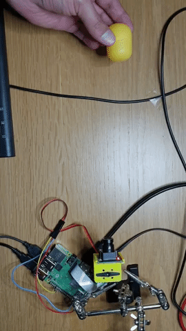
It works reasonably well and the servo keeps the camera pointed towards the yellow ball. I noticed that changing light conditions had an influence on how well the ball is tracked, maybe this something to optimize in the future.
Whats next
I have learned a lot about image processing while doing this project and also saw some other methods (like contour detection) to achieve the same thing. Maybe it would be interesting to also experiment with some other methods and try to determine the pro’s and con’s of the different methods.
Another step would be to try and optimize the process to increase the tracking speed. Normally I prefer using C++ so I might also duplicate the project in C++ and see what the performance difference would be. I have heard many argue that since the Python API is just a wrapper for the C functions the performance increase is not much.
Then there is also the optimization for different light conditions, maybe I can have HSV values for different light conditions and then when no blob is detected it cycles through them…
Something else that could be interesting for the balance robot implementation is to estimate the distance of the ball from the camera. Since I know the actual size of the ball and the size of the reported blob I think it could be possible to estimate a distance, but would need to look into it a bit more.
While reading up and experimenting with blob detection I also found some other interesting applications. One of them is counting objects, since the blob detection function returns a list of detected blobs we can take the length of the list as the number of detected objects. I have actually already implemented this, it’s the value display behind “Count”. Maybe this can also come in handy for future projects.
Anyway the main goal of this sub project was achieved and I can now continue to implement the processes on my balance robot.
This then brings me to the end of this post and I hope you could also find it interesting or useful for your projects.